NeRF - Neural Radiance Fields (review)

Ben Mildenhall\(^{1*}\), Pratul P. Srinivasan\(^{1*}\), Matthew Tancik\(^{1*}\), Jonathan T. Barron\(^2\), Ravi Ramamoorthi\(^3\), Ren Ng\(^1\)
\(^1\) UC Berkeley, \(^2\) Google Research, \(^3\) UC San Diego

We wish to obtain views from new viewpoints of a scene from a set of 2D RGB images (about 20 to 100 images). Figure 1 gives an excellent visual explanation of the task.

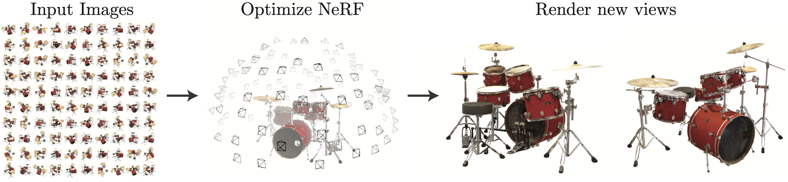
Just to be absolutely clear, I will list down the training data and the output of the task separately:

Training data: A set of \(N_{image}\) (image, viewpoint) pairs for a scene
Output: For any new viewpoint not in the training data, we can obtain the image for the scene as seen from that view

Show-n-tell

Nothing better than seeing some awesome results to motivate this blog! Please see the videos in full-screen mode for a better experience.

What do we mean by viewpoint

A viewpoint means the position of the camera with respect to the scene. Figure 2 shows two different viewpoints as camera\(_1\) and camera\(_2\). Notice that the camera is always at a constant distance \(r\) from the centre of the scene.

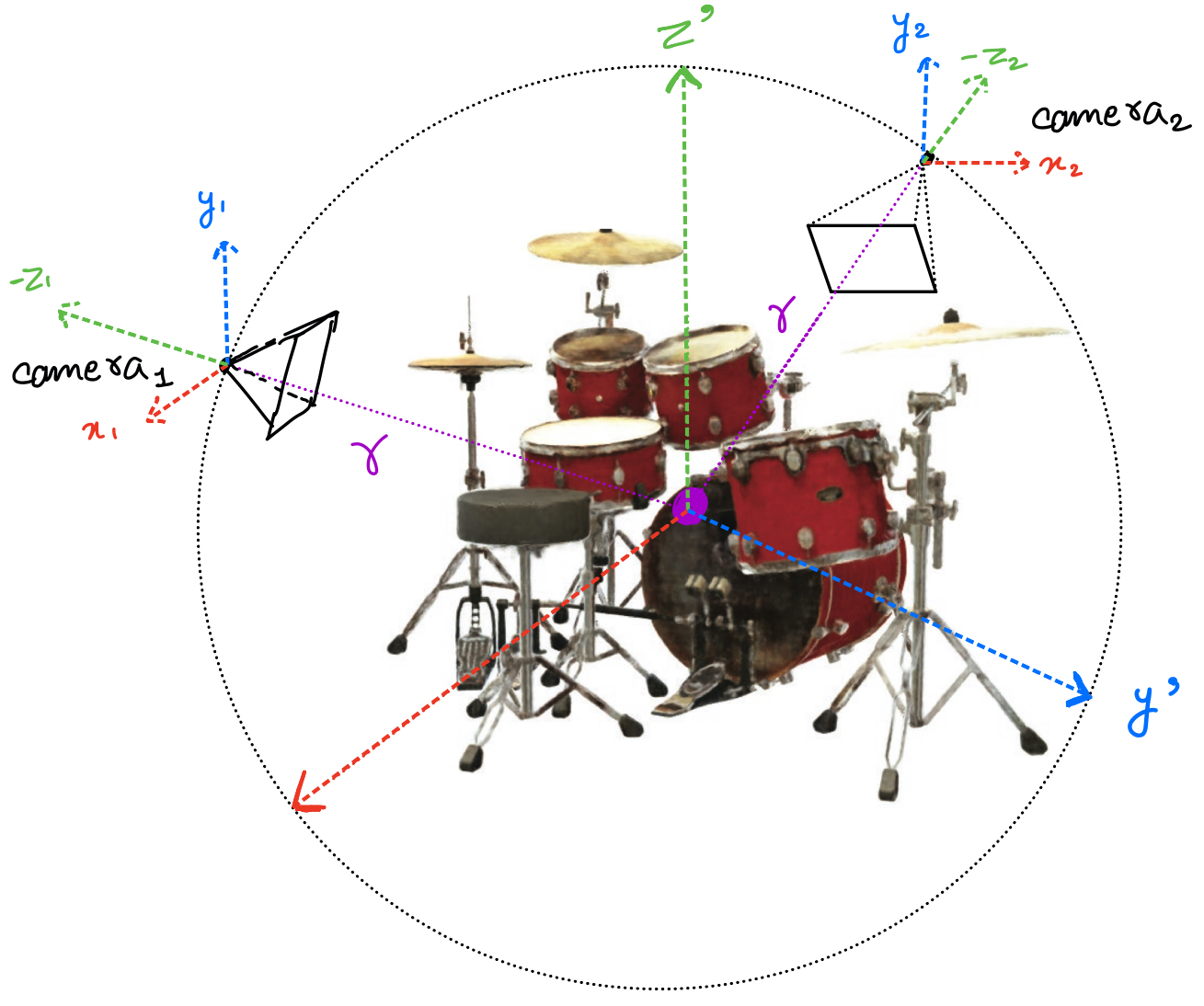
To completely define the viewpoint, we only need to define the angle of the line joining the camera to the centre (since the distance of the camera from the centre is always \(r\)).

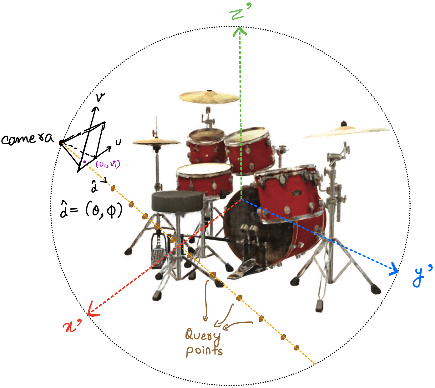
To define the angle of any direction \(\hat{a}\), we only need two angles. \(\theta\) to define its position in the x-y plane. Once its fixed in the x-y plane, we can use another angle \(\phi\) to lift it off the x-y plane towards the z-axis. This is shown in figure 3.

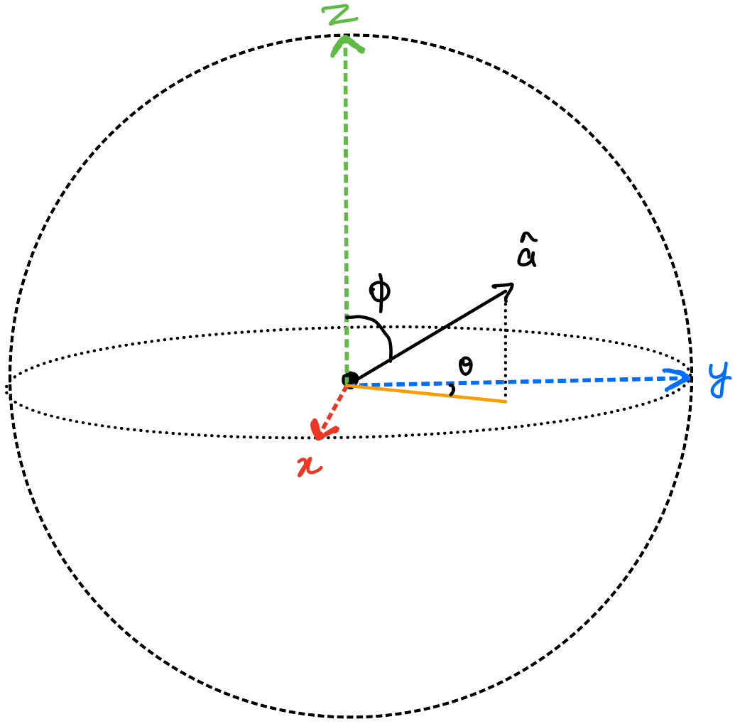
In summary, a direction vector can be completely defined using a \((\theta, \phi)\) pair. In figure 2, by joining the camera\(_1\) to a pixel of the image, we can have a unique direction denoted by a \((\theta, \phi)\) pair. Similarly, we will join the camera to every pixel of the image.

In total, we will have as many \((\theta, \phi)\) pairs as the number of pixels in the image. Each pair will define the direction of the line joining the corresponding pixel to the camera.

Highest level overview

Now that we are clear with the inputs and what we want to achieve, we can start diving into the ‘how’. Figure 4 shows a high-level overview of the method.

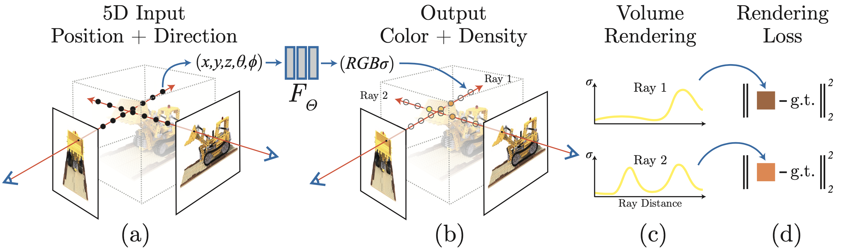
Let’s see a step by step breakdown of how to interpret figure 4. Please refer to figure 5 while reading the description below.

For each pixel \((u_1, v_1)\) of the image:

1. Imagine a ray of light in the \(\hat{d}\) direction emerging from the camera to the pixel. As discussed in the previous section, this direction can be defined using two angles, \(\hat{d} = (\theta, \phi)\).
2. This ray will hit several points of the scene. The colour that we finally observe at \((u_1,v_1)\) in the image will be a combination of the colour of those points and their opacity (how much light they allow to pass through them).
3. We use an equation to combine the colours of all the points along the ray according to their opacity.
4. We compare the calculated value of the colour of the pixel \((u_1, v_1)\) and the actual value from the input image using a loss function.

Now that we have the basic overview of how NeRF works let’s dive into a bit more detail!

Adding details

1. Intuitively, the colour of any point in the scene should depend on where the camera is (shadows, reflection etc). Therefore, the colour is not only a function of the coordinates of the point \((x,y,z)\) but also the direction \(\theta, \phi\) from which we are viewing that point. The figure below depicts the variation in colour of two points, one on the ship and another on the water, as we change viewpoints.
   
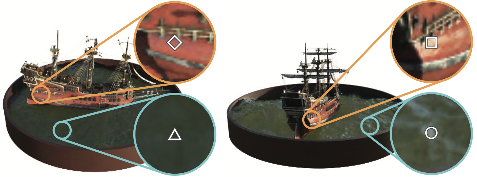   Figure 6 - How the colour of points changes with viewpoint.
2. The amount of light that any point reflects, refracts and transmits is an inherent property of the point and should be independent of the viewpoint. Thus the density \(\sigma\) is only a function of the coordinates \((x,y,z)\).

How to get colour at a point?

As touched upon in points 2 and 3 of the high-level overview, to get the predicted value of any pixel, we need two things -

1. The colour of a point (RGB value)
2. How much light it allows to pass through it (depends on the density \(\sigma\))

And as we discussed in the previous section, the colour is a function of both coordinates and viewpoint \(F_{color}: (x,y,z,\theta,\phi) \rightarrow (R,G,B)\), whereas density only depends on the coordinates \(F_{density}: (x,y,z) \rightarrow \sigma\).

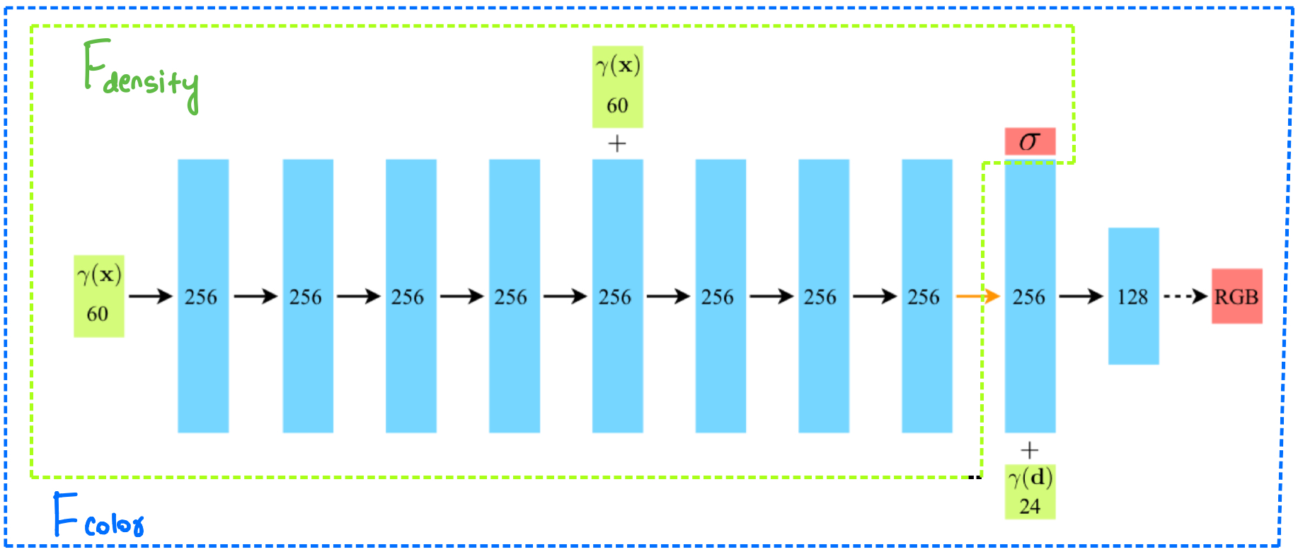
We will now use a fully-connected neural network to approximate the functions \(F_{color}\) and \(F_{density}\). The network architecture is straightforward, just a few fully connected layers. This small network architecture provides a great advantage that we will discuss a little while later.

The notation used in the figure is slightly different, with \(\text{x} = (x,y,z)\) and \(\text{d} = (d_x, d_y, d_z)\) refers to the viewpoint (\(\theta,\phi\)) in cartesian form (we have been using polar form till now, but they are easily interconvertible).
We can again observe in the network architecture figure that \(F_{density}\) (shown in dotted green box) is a function of only position \(\text{x}\) whereas \(F_{color}\) (shown in dotted blue box) is a function of both \(\text{x}\) and the viewpoint \(\text{d}\).

For now, please ignore the \(\gamma\) function and simply treat the green input boxes as \(\text{x}\) and \(\text{d}\). We will come to the gamma function and its use in the next section.

Combining the colours along a ray

Please recall point 3 of the high-level explanation, corresponding to the volume rendering step in figure 4. We now have to combine the different colours of the points (that the ray hits) according to their densities.

Now, I’m going to write a scary (but intuitive) equation that we will use to get the expected colour of a camera ray \(C(\textbf{r})\):

Please note that a complete understanding of this equation will off-road us from the main point of the paper. For the more interested readers, I will be explaining this equation, called the rendering equation, in another blog post.

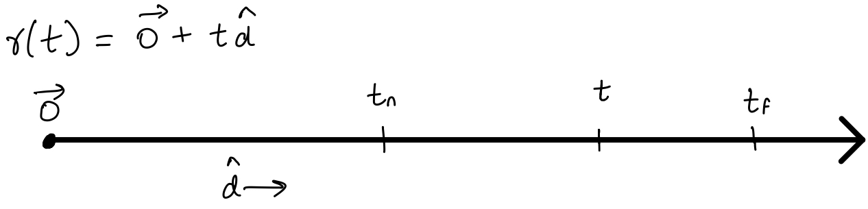
For now, we only need to have an intuitive understanding of the terms here. The input \(\textbf{r}(t) = \textbf{o} + t\textbf{d}\) denotes the camera ray, and can be imagined as just a line. We are only interested in the values of \(t\) from \(t_n\) to \(t_f\) (near and far bounds, the limits of the integral).

Note to keep in mind:
For efficiency reasons, we render the scene from our eyes to the source instead of the other way around. This is called backward tracing, and is almost always used in practice.

So, why do we observe colours? It is because the light from any light source is reflected partially in our direction. Intuitively, the colour that we observe for any object should depend on three factors -

1. The intensity with which the reflected light reaches us (depends on the density of objects in between)
2. The material properties of the object (density) to reflect light
3. The colour of the reflected light in the our direction

The function \(\textcolor{red}{T(t)}\) denotes the accumulated transmittance along the ray from \(t_n\) to \(t\). As expected, the actual function is a function of the densities of the points in between.

The volume density \(\textcolor{green}{\sigma(\textbf{r}(t))}\) can be interpreted as the differential probability of a ray terminating at an infinitesimal particle at location \(\textbf{r}(t)\).

The term \(\textcolor{blue}{\textbf{c}(\textbf{r}(t), \textbf{d})}\) means the total radiance(light) that the point at \(t\) of \(\textbf{r}(t)\) sends in the direction \(d\). Due to reversibility, it is better to think of it light in the \(- \hat{d}\) direction towards \(\textbf{o}\).

And now, as promised, here’s the blog on the fun physics behind the rendering equation!

Integral as a sum

Intuition of the equation?
Let us see how to evaluate the rendering equation. We replace the integral with a sum over some chosen discrete points between \(t_n\) and \(t_f\):

where \(\delta_i = t_{i+1} - t_i\) is the distance between adjacent samples, and is the replacement for \(dt\) in the original equation.

Discrete sampling

The last question that we wish to answer is how to sample points in [\(t_n, t_f\)] for evaluating the sum.

NeRF uses a stratified sampling approach (Wikipedia), which is jargon for dividing the population into bins and sampling uniformly from the bins. The advantage of stratified sampling is that it ensures that each bin has some representation in the final answer.

Here is the same thing, but in math. Here N denotes the number of bins and one point is being sampled uniformly from each bin:

Summary till now

We can now sample points in a range and use the rendering equation to combine the colours of these points. Doing this will give us the predicted colour value of a pixel. We can then apply our \(L_2\) loss with the actual pixel colour. What’s the problem?

Clever tricks

1. Hierarchical sampling

Well, it turns out that with typical large values of the number of points sampled, \(N = 256\), the rendering strategy is inefficient: free space and occluded regions do not contribute to the rendered image yet they are sampled repeatedly.

To increase efficiency, NeRF uses a two-step hierarchical approach to sampling that increases rendering efficiency. The motivation in breaking down sampling to a two-step process is that we wish to allocate samples proportionally to their expected effect on the final rendering.

In the first coarse pass, we will sample a small number of points \(N_c\) using the naive stratified sampling. This pass will tell us the regions where good points lie.

In the second fine pass, we will use the regions where the good points lie to sample more points \(N_f\). To do this, we will treat normalize \(\hat{w_i} = w_i/\sum_{j = 0}^{N_c}{w_j}\). These normalized weights produce a piecewise-constant PDF along the ray. We sample the second set of \(N_f\) locations from this distribution, evaluate our “fine” network at the union of the first and second set of samples, and compute the final rendered colour of the ray using all \(N_c + N_f\) samples.

Note that NeRF simultaneously optimizes two networks: one coarse and one fine.

2. Positional encoding

Let us come to a neat little trick that NeRF uses. The motivation is that the scenes are complex functions. To reconstruct such scenes, the neural network needs to be able to approximate high-frequency functions. Neural networks in their raw form are not so good at doing this [2]. The paper suggests that after mapping the 5D input (\(x, y, z, \theta, \phi\)) to a high-dimensional representation, the neural network is better able to approximate high-frequency functions.

Let’s first see how the positional encoding is used:

For any scalar \(p\), the function \(\gamma(p)\) converts it into a \(2L\)-dimensional representation.

All this is well and good, but is this really important? Boy, you’re in for a surprise! Let’s compare the results with and without using the positional encoding:

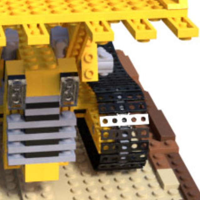
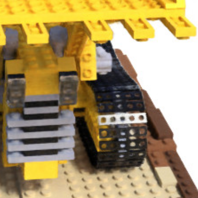
The idea of positional encoding is not new. It is already widely used in NLP, specifically Transformers. However, the drastic improvement here is quite astonishing to me!

Results and comparisons

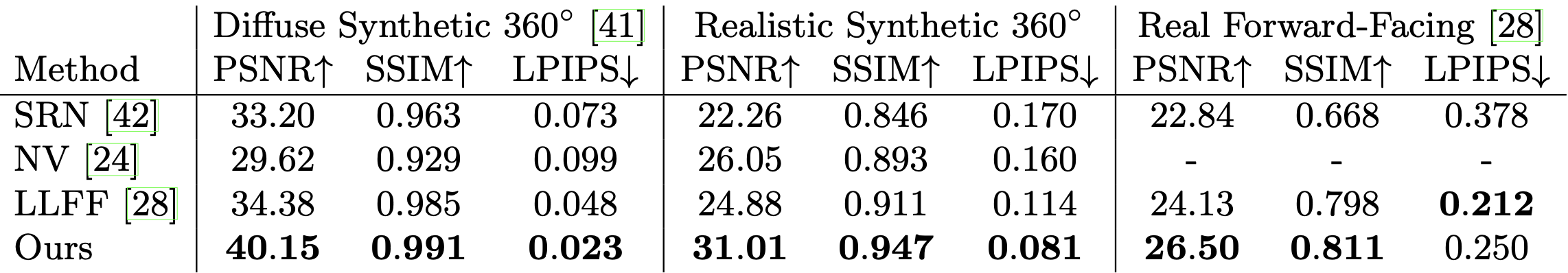
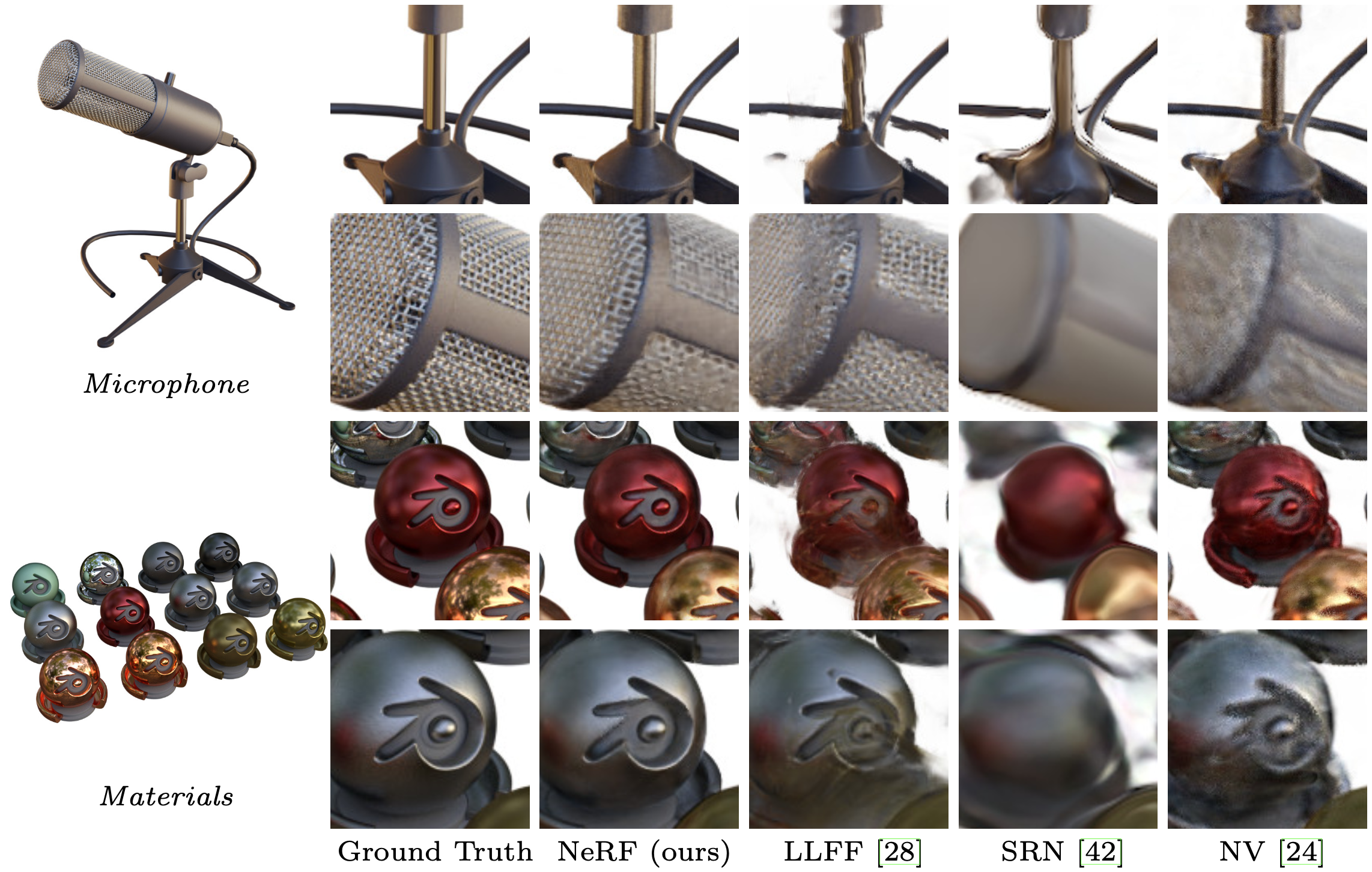
Merits

• high-quality state-of-the-art reconstructions
• does a great job with occluded objects and reflections from surfaces
• accurate depth information for any view can be extracted using \(\sigma\) of each coordinate
• 3D representation size is ~5MB, which is lesser than the storage required to store the raw images alone!

De-merits

• the network is trained separately for each scene
• training takes at least 10 hours for a single scene
• without the positional encoding, the quality of the reconstructions seems to dwindle drastically

Implementations

1. Official code (tensorflow)
2. Other pytorch and tensorflow implementations

References

1. NeRF: Representing Scenes as Neural Radiance Fields for View Synthesis [Arxiv]
2. Fourier Features Let Networks Learn High Frequency Functions in Low Dimensional Domains [Arxiv]
3. Two minute papers video!
4. Project page
5. ECCV 2020 short (4-minute) and long (10-minute) talk
6. Blogs on nerfs (1, 2)
7. An excellent explanation of the basics of ray tracing

Media sources

1. From paper: Figure 1, 4, 6, 7, 9, 10, 11, 12
2. From project website: Videos
3. Mine: Figure 2, 3, 5, 8

Feedback is highly appreciated so I can improve this (and future) posts. Please leave a vote and/or a comment (anonymous comments are enabled)!